Handling diverse filetypes in Pandas

Last updated on 2025-06-12 | Edit this page

Overview

Questions

How can I read in different tabular file formats to a familiar data type in Python?
What are some common errors that occur when importing data, and how can I troubleshoot them?

Objectives

Import tabular data from Excel, JSON, XML and Parquet formats to pandas dataframes using the pandas library
Use help and function documentation to select and set parameters in function calls.

Untangling a data pile

To illustrate the centrality of these problems, let’s imagine the following scenario:

You’re poking around your research lab’s collaborative drive when you find a folder containing data, code and some notes from a former postdoctoral researcher. They were investigating patterns in the emissions intensity of electricity production in Puerto Rico as exploratory work for a potential research project, but wound up pursuing another idea instead.

As you prepare for your qualifying exams, you’re interested in picking up on their work and developing it further. You find the data folder that the postdoc was using to store data inputs to his model. It’s a bit of a mess!

Every file in the folder has the same name (“eia923_2022”) but a different file extension. To make sense of this undocumented pile of files, we’ll need to read in each file and compare them.

EIA 923 data

The Energy Information Administration (EIA)’s Form 923 is known as the Power Plant Operations Report. The data include electric power generation, energy source consumption, end of reporting period fossil fuel stocks, as well as the quality and cost of fossil fuel receipts at the power plant and prime mover level (with a subset of +10MW steam-electric plants reporting at the boiler and generator level). Information is available for non-utility plants starting in 1970 and utility plants beginning in 1999. The Form EIA-923 has evolved over the years, beginning as an environmental add-on in 2007 and ultimately eclipsing the information previously recorded in EIA-906, EIA-920, FERC 423, and EIA-423 by 2008.

Given your interest in generation and fuel consumption data for your research, the EIA Form 923 data is a great starting point for data exploration.

Get ready

Open up the notebook for this lesson by running

BASH

$ uv run jupyter notebook

from the open-energy-data-for-all directory. Then in the Jupyter browser, open notebooks/2-diverse-filetypes.ipynb.

Reading Excel files with Pandas

One of the most popular libraries used to work with tabular data in Python is called the Python Data Analysis Library (or simply, Pandas). Pandas has functions to handle reading in a diversity of file types, from CSVs and Excel spreadsheets to more complex data formats such as XML and Parquet. Each read function offers a variety of parameters designed to handle common complexities specific to the file type on import. For a refresher on Pandas, Pandas DataFrames and reading in files, see the Starting with Data lesson.

Callout

Identifying file paths

In order to read data into Pandas or any Python function, we’ll need to identify the path to that file. The path tells the code where that file lives. There are two ways to specify the path to any file on your computer:

Absolute path: An absolute path specifies a location from the root of the filesystem.
Relative path: A relative path specifies a location starting from the current location. The relative path is just a subset of the absolute path.

For example, to get to the eia923_2022.json file in the data folder from a notebook in the open-energy-data-for-all folder, we can either specify:

Absolute path: /home/user/Desktop/path/to/open-energy-data-for-all/folder/data/eia923_2022.json
Relative path: data/eia923_2022.json

Handling spreadsheet formatting on read-in

Of all the files in the data folder, you decide to start with the Excel spreadsheet. To read in an Excel spreadsheet using pandas, you will use the read_excel() function:

PYTHON

import pandas as pd
pd.read_excel('data/eia923_2022.xlsx')

That took a while! Luckily,read_excel() offers built-in functionality to handle various Excel formatting challenges. Let’s see if there’s a way to quickly explore a smaller subset of the data. While we can always look up documentation online, we can also access a function’s documentation right in Python. To identify which parameter might be able to help us, we can use the help() function to pull up the function documentation:

PYTHON

help(pd.read_excel)

For each parameter, the documentation provides the name of the parameter, the format for the parameter input (e.g., list, string, int), the default value if no value is provided, and an explanation of what the parameter does.

We can see that the nrows parameter provides the following documentation:

OUTPUT

nrows : int, default None
    Number of rows to parse.

So, if we only want to parse the first 100 rows of the data, we can call:

PYTHON

pd.read_excel('data/eia923_2022.xlsx', nrows=100)

That’s better. But unfortunately, something doesn’t look quite right! When opening the file in a spreadsheet software, you see that the first few rows look like this:

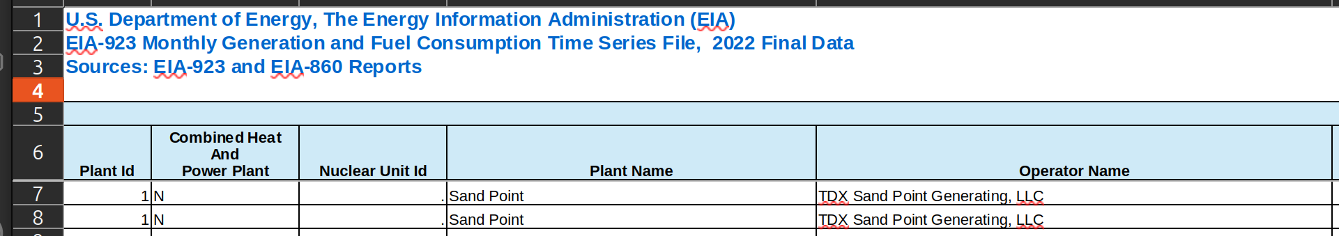
Snapshot of the Excel file showing the first 6 rows contain metadata, blank spaces and column names.

To read the spreadsheet in correctly, we want to ignore these first five rows.

Challenge

Challenge 1: handling Excel formatting on read-in

Looking at the documentation for pd.read_excel(), identify the parameter needed to ignore the first few rows of the spreadsheet. Then, using pd.read_excel(), read in the eia923_2022.xlsx file using this parameter to skip any rows that don’t contain the column headers. Store the result in a variable called eia923_excel_df.

Show me the solution

PYTHON

import pandas as pd

eia923_excel_df = pd.read_excel('data/eia923_2022.xlsx', skiprows=5)

Each row contains monthly generation data for each plant’s prime mover. While a subset of plants fill out Form 923 at the boiler and generator, a large proportion of plants only report at this more aggregated level. For more on the nuances of the Form 923 data, see PUDL’s data source page for EIA-923.

Reading in JSON files

JavaScript Object Notation (JSON) is a lightweight file format based on name-value pairs, similar to Python dictionaries. JSON is often used to send data to and from web applications, and is one of the most common formats available when you’re accessing data from an Application Programming Interface (API). JSON data can be found saved as either .json or .txt files.

Nested content in JSON files

Pandas read_*() methods assume tabular data. When a JSON file represents a table and nothing else, we can use pd.read_json() to read it in directly. Most often, we know a JSON file contains a table when we see a list of dictionaries, or a dictionary of lists.

However, JSON is a flexible format, and JSON files can be organized all kinds of ways. Unlike Excel or CSV spreadsheets, many JSON files don’t just contain a table. Instead, most JSONs contain data in a nested format.

Nested JSON contains multiple levels of data:

OUTPUT

{
  "response": {
    "data": [
      {
        "period": "2022-12",
        "plantCode": "6761"
      },
      {
        "period": "2022-12",
        "plantCode": "54152"
      }
    ]
  }
}

To successfully extract tabular data from nested JSON, we need to identify which part of the structure contains the tabular data we’re looking for. Here, the response contains another name-value pair called data, and data contains a list with two records, each of which has two name-value pairs (period and plantCode).

The data contained in this JSON file can be represented as a table! In this case, each dictionary corresponds to one row of the data, and each name (e.g., “period”) corresponds to a column name. This is the “list of dictionaries” approach to expressing a table in JSON format that we mentioned above.

Callout

JSONs can include many levels of nesting, including different levels of nesting for similar records or other formatting that doesn’t obey the principles of tabular structure (where each row represents a single record, and each column represents a single variable). We focus on extracting tabular data from these nested JSONs in this lesson, but some JSON files may not contain tabular data at all.

Reading in JSON files using `json.load()`

To better visualize our JSON file, let’s read it into Python without changing its format. To do this, we use the json package, and the load method.

While Pandas handles opening a file in the read_*() methods, json.load() does not - so, we first need to read the file into Python. To do so, we use the open() function.

Callout

When we open() a file in Python, we should always close it after we’ve extracted the data we need. Closing a file frees up system resources and ensures that we aren’t accidentally modifying our original file.

To automatically handle file opening and closing, we use a context manager. Using the word with, we put all the code we want to run on the opened file into an indented block.

PYTHON

import json
with open('data/eia923_2022.json') as file:
    eia923_json = json.load(file)

eia923_json

The first part of the result looks like this:

OUTPUT

{'response': {'warnings': [{'warning': 'incomplete return',
    'description': 'The API can only return 5000 rows in JSON format.  Please consider constraining your request with facet, start, or end, or using offset to paginate results.'},
   {'warning': 'another warning', 'description': 'Hey! Watch out!'}],
  'total': '6949',
  'dateFormat': 'YYYY-MM',
  'frequency': 'monthly',
  'data': [{'period': '2020-11',
    'plantCode': '61034',
    'plantName': 'EcoElectrica',
    'fuel2002': 'ALL',
    'fuelTypeDescription': 'Total',
    'state': 'PR',
    'stateDescription': None,
    'primeMover': 'ALL',
    'generation': '299985',
    'gross-generation': '314449',
    'generation-units': 'megawatthours',
    'gross-generation-units': 'megawatthours'},
    ...

By using json.load(), we’ve read our file into a Python dictionary. Now, we can use .keys() to see a list of all the keys in the first level of the dictionary - this is a quick and helpful way to get a sense for what is contained in different parts of the JSON file, without having to scroll through the entire output.

To see the value of any particular key, we can call it in square brackets by name:

PYTHON

eia923_json['response']

This returns yet another dictionary with a list of keys. To look more closely at the warnings the file contains, we can add another square bracket:

PYTHON

eia923_json['response']['warnings']

OUTPUT

[{'warning': 'incomplete return',
  'description': 'The API can only return 5000 rows in JSON format.  Please consider constraining your request with facet, start, or end, or using offset to paginate results.'},
 {'warning': 'another warning', 'description': 'Hey! Watch out!'}]

Now that we’ve found the path to our data table in the JSON file, we can use pd.DataFrame() to transform it into a Pandas DataFrame:

PYTHON

pd.DataFrame(eia923_json['response','warnings'])

The function returns a DataFrame that looks like this:

OUTPUT

|           warning |                                       description |
|------------------:|--------------------------------------------------:|
| incomplete return | The API can only return 5000 rows in JSON form... |
|   another warning |                                   Hey! Watch out! |

The first row of this table is letting us know that when the postdoc queried and saved this data from the API, he only got the first 5,000 rows of data. We’ll tackle this problem in a later episode, but for now let’s investigate the data that we do have saved locally.

Challenge

Challenge 2: find that table!

Fill in the blanks in the code below to read in the data from the eia923_2022.json file into a Pandas DataFrame.

PYTHON

with open('data/eia923_2022.json') as file:
    eia923_json = ...

eia923_json_df = pd.DataFrame(eia923_json[...])

Give me a hint

First, read in the file using open() and json.load(). Once you’ve read in the file, you can iterate through the .keys() of the dictionary to find the path to the data portion of the file.

Show me the solution

PYTHON

import pandas as pd
import json

import json
with open('data/eia923_2022.json') as file:
    eia923_json = json.load(file)

eia923_json_df = pd.DataFrame(eia923_json['response']['data'])

Deciphering XML

eXtensible Markup Language (XML) is a plain text file that uses tags to describe the structure and content of the data they contain. For example, the following might be a way to represent a note from Saul R. Panel to Dr. Watts apologizing for leaving the project in an incomplete state:

XML

<note>
  <from>Saul R. Panel</from>
  <to>Dr. Watts</to>
  <heading>Note about project</heading>
  <body>Sorry for leaving the project in an incomplete state!</body>
</note>

In JSON, the equivalent information could be formatted as:

OUTPUT

{
  "note": {
    "from": "Saul R. Panel",
    "to": "Dr. Watts",
    "heading": "Note about project",
    "body": "Sorry for leaving the project in an incomplete state!"
  }
}

Like other markup languages (e.g., HTML), XML wraps around data, providing information about the structure, format, and relationships between components. Each tag provides metadata about what the piece of data it contains represents - for instance <row> will contain a row of data, while <plantCode>243</plantCode> will means that the plant code is 243.

Each tag in XML shares similarities with a key in a JSON file: - both provide metadata about what the corresponding value is (e.g., a note, net generation in watts) - both provide information about nested relationships (e.g., the note contains a heading and a body)

However, unlike JSON, XML tags: - can have additional attributes (e.g., <data type="float" precision=3 variable_name="net-generation-mw">3.142</data>), providing a way to share more complex metadata about a given data point and to search for tags matching additional filters (e.g., all data with a particular variable name).

While XML is harder and slower to read than JSON, it also has more capabilities. You might be likely to see an XML file if the data you’re looking at:

is old! XML was invented in 1998 and is still widely in use in older data distribution methods.
has deeply nested hierarchies of relationships, like FERC’s accounting data.
is large and complex! For instance, JSON can only handle strings, numbers and booleans, while XML can also be used to share images, charts and graphs.
is distributed through an RSS feed. For instance, FERC publishes filings on a rolling basis using an RSS feed and the XML data format.

Using `pd.read_xml()`

Like with our other data types, we can use pd.read_xml() to parse XML files into Pandas DataFrames. pd.read_xml() is designed to ingest tabular data nested in XML files, not to coerce highly nested data into a table format. To use this method, we’ll need to identify where in our XML file the data is structured into a table-like format and can be easily extracted to a DataFrame. For more on pd.read_xml(), see the Pandas documentation.

Let’s try to explore the XML file that the postdoc left behind:

PYTHON

pd.read_xml('data/eia923_2022.xml')

Hm, that doesn’t look quite right. Each tag has been assigned as a column name, and the value inside has been added as a row.

If we open up the XML file in a text editor or browser, we can see that a nested series of tags can help us identify the part of the table we want to read in.

XML

<response>
    <warnings>
        <row>
            <warning>incomplete return</warning>
            <description>The API can only return 300 rows in XML format.  Please consider constraining your request with facet, start, or end, or using offset to paginate results.</description>
        </row>
        <row>
            <warning>another warning</warning>
            <description>Hey! Watch out!</description>
        </row>
    </warnings>
    <total>6949</total>
    <dateFormat>YYYY-MM</dateFormat>
    <frequency>monthly</frequency>
    ...

For example, the same warnings table we were working with before is in the tag, then the tag. Each row of the data is also wrapped in a tag.

To drill down to the section of the file we are actually interested in, we can use the xpath parameter, which lets you use tags to specify where in the XML file to look for a table.

The xpath query we’re looking for is formatted as follows:

// are used at the beginning to note that we want to select all items with the tags specified
Then, like specifying which directory we want to access in a terminal, slashes are used to specify the path to the desired tag.

So to get all the <row>s of the <warnings> table, we call:

PYTHON

pd.read_xml('data/eia923_2022.xml', xpath = "//response/warnings/row")

Challenge

Challenge 3: Reading in XML data

Read in all the rows of the data table in eia923_2022.xml into a Pandas DataFrame, using pd.read_xml and the xpath parameter. Store the result in a variable called eia923_xml_df.

Show me the solution

PY

eia923_xml_df = pd.read_xml('data/eia923_2022.xml', xpath = "//response/data/row")

The data is found following the following tags: <response><data><row>

The <data> is split into two seperate chunks of data seperated by <row> tags, which tells us that everything between these tags corresponds to a single row of data. Then, we know that the <period>, <plantCode> and <plantName> tags are telling us what variable the values correspond to - or in other words, what the column name is that corresponds to each tag. We use the xpath parameter to grab all <row>’s of data in the XML file.

Callout

xpath can be used to make more complex queries (e.g., only picking <note>’s written after a certain date), but we won’t cover more advanced usage of xpath in this tutorial. See this Library Carpentries tutorial for more about xpath.

`pd.read_parquet()`

There’s one more file left in the data folder the postdoc left behind - a Parquet file! You can think of Parquet files as spreadsheet storage optimized for computers. Like an Excel file, it’s very difficult for a human to read the plain text of the file, as it is designed to be read efficiently by software.

Parquet files: - are designed to efficiently process and store large volumes of data, making them about 50x faster than using pd.read_csv() on comparable file sizes. - are saved with data organized into chunks (e.g., one chunk per month), making it possible to quickly load data from some part of the dataset without loading everything into memory. - are supported by many existing tools, including Pandas.

Callout

To get into the technical weeds of Parquet files, see the Parquet documentation. For a desktop viewer similar to Excel, we recommend checking out Tad.

We can read a Parquet file to a Pandas DataFrame using pd.read_parquet(), almost identical to how we would read in a CSV:

PY

eia923_parquet_df = pd.read_parquet('data/eia923_2022.parquet')

Challenge

Challenge 4: Comparing datasets

Pick two datasets we’ve just read in, and compare them. How are they similar, and how are they different? Share your reflections with a peer.

Give me a hint

df.info() provides a high level summary of the data, including the columns available, their data types, the number of non-null values in each column, and the overall number of rows in the DataFrame.
Inspect a column in a DataFrame df by using df[column_name].
To quickly see what values are contained in a column, you can use df[column_name].unique() to get a list of unique values in the column.
Try using df.iloc[0] to get the values from the first row of the data.
df.head(n) returns the first n rows of the data, and df.tail(n) returns the last n rows.

Key Points

pandas has functionality to read in many data formats (e.g., XML, JSON, Parquet) into Pandas DataFrames in Python. We can take advantage of this to transform many kinds of structured and semi-structured data into similarly formatted data.
The help function can be used to access function documentation, providing avenues to resolve problems on import of various data types.
When semi-structured data contains tabular data, we can extract the tabular data into a Pandas Dataframe.

Handling diverse filetypes in Pandas

Overview

Questions

Objectives

Untangling a data pile

EIA 923 data

Get ready

BASH

Reading Excel files with Pandas

Identifying file paths

Handling spreadsheet formatting on read-in

PYTHON

PYTHON

OUTPUT

PYTHON

Challenge 1: handling Excel formatting on read-in

Show me the solution

PYTHON

Reading in JSON files

Nested content in JSON files

OUTPUT

Reading in JSON files using json.load()

PYTHON

OUTPUT

PYTHON

PYTHON

OUTPUT

PYTHON

OUTPUT

Challenge 2: find that table!

PYTHON

Give me a hint

Show me the solution

PYTHON

Deciphering XML

XML

OUTPUT

Using pd.read_xml()

PYTHON

XML

PYTHON

Challenge 3: Reading in XML data

Show me the solution

PY

pd.read_parquet()

PY

Challenge 4: Comparing datasets

Give me a hint

Reading in JSON files using `json.load()`

Using `pd.read_xml()`

`pd.read_parquet()`